
First, start an ipython sesion in pylab mode:
$ ipython --pylab
This will automatically load numpy and matplolib and enable the interactive plotting environment.
Once ipython is running, you can import the cosmicpy package:
In [1]: from cosmicpy import *
The next step is to create a cosmology object. Let us start with a default cosmology:
In [2]: cosmo = cosmology()
To get a summary of the cosmological parameters defined in this object, you can use the print() fucntion:
In [3]: print cosmo
FLRW Cosmology with the following parameters:
    h:        0.7
    Omega_b:  0.045
    Omega_m:  0.25
    Omega_de: 0.75
    w0:       -0.95
    wa:       0.0
    n:        1.0
    tau:      0.09
    sigma8:   0.8
All the cosmological parameters are accessible as attributes of the cosmology object. For instance, to check the value of the matter density today \(\Omega_m\) run:
In [4]: cosmo.Omega_m
Out[4]: 0.25
The values for the cosmological parameters can be modified which will automatically trigger an update of all the derived quantities.
To illustrate this, let’s see the value of the sound horizon at recombination \(s_h\) with the default cosmology, update \(\Omega_m\) and check that the value of \(s_h\) has changed:
In [5]: cosmo.sh_r
Out[5]: 105.27381988350771

In [6]: cosmo.Omega_m = 0.3

In [7]: cosmo.sh_r
Out[7]: 100.59308203228834
The cosmological parameters can also be set at the creation of the cosmology object by specifying their values to the constructor. For instance, to create a cosmology with \(\Omega_m = 0.2\) and \(\Omega_{de} = 0.8\):
In [8]: cosmo2 = cosmology(Omega_m=0.2, Omega_de=0.8)

In [9]: print cosmo2
FLRW Cosmology with the following parameters:
    h:        0.7
    Omega_b:  0.045
    Omega_m:  0.2
    Omega_de: 0.8
    w0:       -0.95
    wa:       0.0
    n:        1.0
    tau:      0.09
    sigma8:   0.8
Now that we have seen how to create a cosmology object with the desired cosmological parameters, let’s use it to compute some distances.
cosmology offers a number of different methods to compute various cosmological distances:
| cosmology.a2chi(a) | Radial comoving distance in [Mpc/h] for a given scale factor. |
| cosmology.f_k(a) | Transverse comoving distance in [Mpc/h] for a given scale factor. |
| cosmology.d_A(a) | Angular diameter distance in [Mpc/h] for a given scale factor. |
These methods all compute a distance as a function of the scale factor \(a\).
It is often usefull to work with redshifts instead of scale factors. The conversion between the two quantities is performed by the 2 utility functions:
| cosmicpy.utils.z2a(z) | converts from redshift to scale factor |
| cosmicpy.utils.a2z(a) | converts from scale factor to redshift |
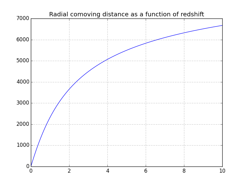
Here is an example to compute the radial comoving distance for an array of redshifts between 0 and 10:
In [10]: z = arange(0,10,0.01)

In [11]: figure();

# The z2a function is used to convert z to scale factors
In [12]: plot(z,cosmo.a2chi(z2a(z))); grid();

In [13]: title('Radial comoving distance as a function of redshift');
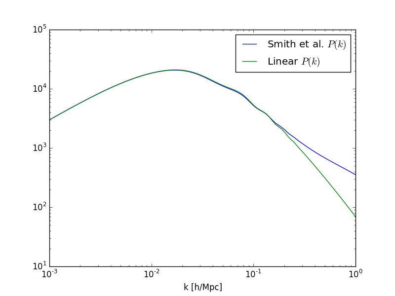
cosmology implements several methods to compute the linear and non linear matter power spectrum:
| cosmology.pk_lin(k[, a]) | Computes the linear matter power spectrum. |
| cosmology.pk(k[, a, nl_type]) | Computes the full non linear matter power spectrum. |
By default, these two functions will compute the power spectrum at \(a=1\) and using the Eisenstein & Hu transfer function with oscillations. The non-linear correction implemented in cosmology.pk() is computed based on [SmithPeacockJenkins+03].
Here is an example to compute these two power spectra:
# Creating a vector of wavenumbers
In [14]: k = logspace(-3,0,100)

In [15]: loglog(k,cosmo.pk(k), label='Smith et al. $P(k)$');

In [16]: loglog(k,cosmo.pk_lin(k), label='Linear $P(k)$');

In [17]: legend(); xlabel('k [h/Mpc]');
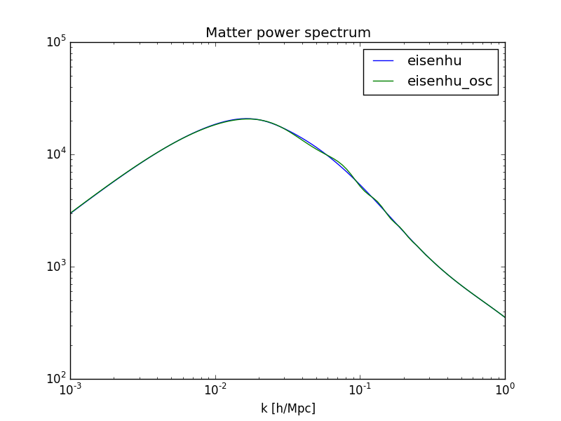
Both power spectra can be computed with or without baryonic oscillations by setting the type keyword to either:
This example shows the matter power spectrum, with non-linear corrections, with and without BAO wiggles:
In [18]: loglog(k, cosmo.pk(k, type='eisenhu'), label='eisenhu');

In [19]: loglog(k, cosmo.pk(k, type='eisenhu_osc'), label='eisenhu_osc');

In [20]: legend(); xlabel('k [h/Mpc]'); title('Matter power spectrum');
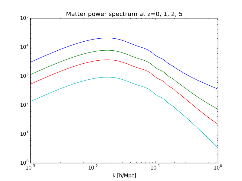
Finally, the power spectrum can be computed at different scale factors:
# Create an array of scale factors corresponding to z=0, 1 ,2 and 5
In [21]: a = z2a(array([0, 1, 2, 5]))

In [22]: loglog(k, cosmo.pk(k,a));

In [23]: xlabel('k [h/Mpc]'); title('Matter power spectrum at z=0, 1, 2, 5');
| [SmithPeacockJenkins+03] | R. E. Smith, J. A. Peacock, A. Jenkins, S. D. M. White, C. S. Frenk, F. R. Pearce, P. A. Thomas, G. Efstathiou, and H. M. P. Couchman. Stable clustering, the halo model and non-linear cosmological power spectra. MNRAS, 341:1311–1332, June 2003. arXiv:astro-ph/0207664, doi:10.1046/j.1365-8711.2003.06503.x. |