In this tutorial, we recover the results of [2012:Rassat] using cosmicpy.
For this tutorial, we are going to use galaxy surveys following a Gaussian selection function of the form:
We define 2 such surveys, one shallow with \(r_0 = 100 \quad h^{-1}\) Mpc and one deep with \(r_0 = 1400 \quad h^{-1}\) Mpc:
In [1]: from cosmicpy import *

In [2]: cosmo = cosmology()

In [3]: surv_deep = survey(nzparams={'type':'gaussian', 'cosmology':cosmo, 'r0':1400}, zmax=3.0, fsky=1.0)

In [4]: surv_shallow = survey(nzparams={'type':'gaussian', 'cosmology':cosmo, 'r0':100}, zmax=0.5, fsky=1.0, chicut=0)
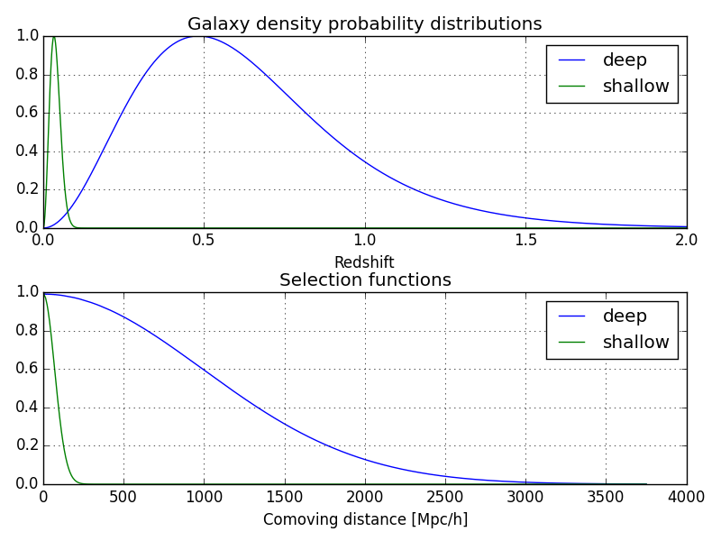
Now, we plot the selection functions along with the galaxy density probability distribution for these 2 surveys normalized by their maximum values:
# Create an array of sampling redshifts between z=0 and z=2
In [5]: z = arange(0.0001,2.0,0.001)

# Convert redshift array into comoving distance
In [6]: r = cosmo.a2chi(z2a(z))

# Compute n(z) for both survey
In [7]: pzd = surv_deep.nz(z)

In [8]: pzs = surv_shallow.nz(z)

# Compute selection function for both survey
In [9]: phid = surv_deep.phi(cosmo,r)

In [10]: phis = surv_shallow.phi(cosmo,r)
Now, let us plot the selection functions and galaxy distributions for both surveys:
In [11]: figure();

In [12]: subplot(211); xlabel('Redshift'); grid();

In [13]: plot(z,pzd/pzd.max(),label='deep');

In [14]: plot(z,pzs/pzs.max(),label='shallow');

In [15]: legend(); title('Galaxy density probability distributions');

In [16]: subplot(212); xlabel('Comoving distance [Mpc/h]'); grid();

In [17]: plot(r,phid/phid.max(),label='deep');

In [18]: plot(r,phis/phis.max(),label='shallow');

In [19]: legend(); title(r'Selection functions');
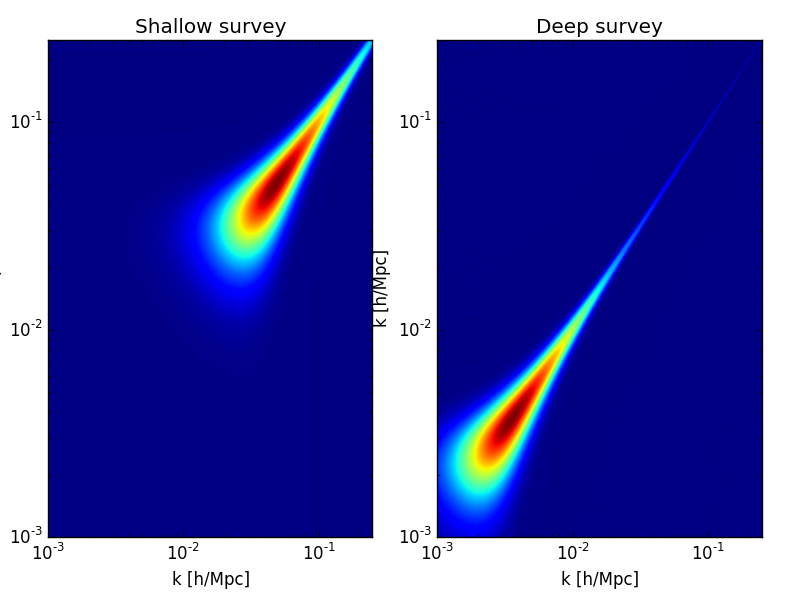
The depth of the survey directly impacts the SFB window function \(W_\ell(k, k')\) : the deeper the survey, the closer to a Dirac \(\delta(k - k')\) it becomes. We illustrate this by computing the window function for \(\ell = 3\) for the 2 surveys we consider using spectra.W() :
In [20]: k = logspace(-3,log(0.25)/log(10),512)

In [21]: sp_deep = spectra(cosmo,surv_deep)

In [22]: sp_shallow = spectra(cosmo,surv_shallow)

In [23]: subplot(121); xscale('log') ; yscale('log')

In [24]: contourf(k, k, sp_shallow.W(3, k, k), 256);

In [25]: title('Shallow survey'); xlabel('k [h/Mpc]'); ylabel('k [h/Mpc]');

In [26]: subplot(122); xscale('log') ; yscale('log')

In [27]: contourf(k, k, sp_deep.W(3, k, k), 256);

In [28]: title(r'Deep survey'); xlabel('k [h/Mpc]'); ylabel('k [h/Mpc]');
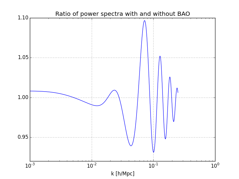
To emphasize the BAO features on the power spectrum, we can plot the ratio of linear power spectra today with and without BAOs. The fitting formulae used here are taken from [EisensteinHu98] . The 2 kinds of power spectra are easily computed using the cosmology.pk_lin() method:
In [29]: pk_osc = cosmo.pk_lin(k,1.0,type='eisenhu_osc')

In [30]: pk = cosmo.pk_lin(k,1.0,type='eisenhu')

In [31]: figure(); grid();

In [32]: semilogx(k,pk_osc/pk);

In [33]:  xlabel('k [h/Mpc]'); title('Ratio of power spectra with and without BAO');
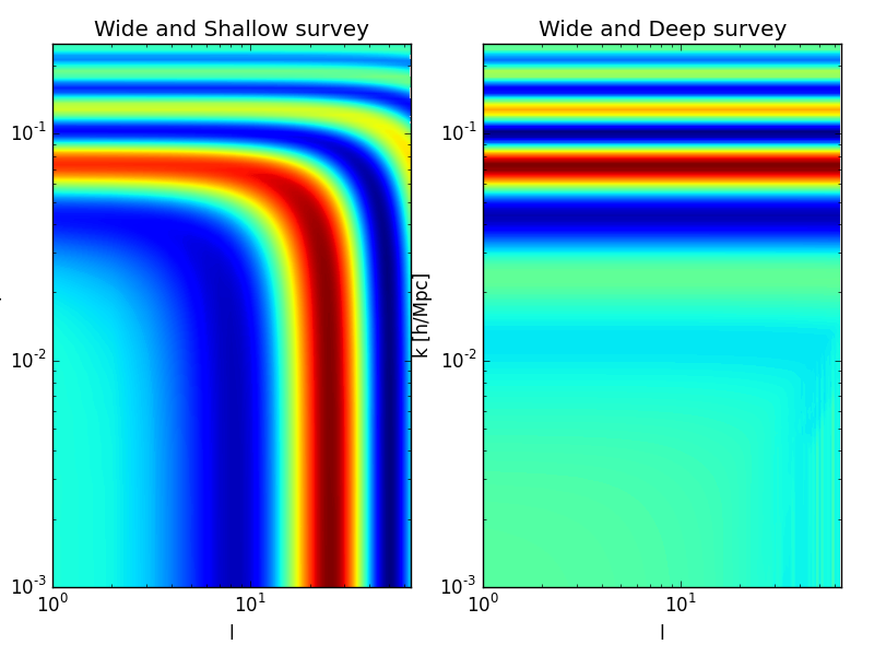
In Spherical Fourier-Bessel space, we consider the ratio \(R_\ell^C (k)\) giben by:
where \(C_\ell^\mathrm{b}(k)\) is the diagonal SFB power spectrum including the physical effects of baryons and \(C_\ell^\mathrm{nob}(k)\) is the smooth part of the SFB power spectrum. Here we use the spectra.cl_sfb() method:
In [34]: k = logspace(-3,log(0.25)/log(10),100)

In [35]: l = arange(1,65)

In [36]: R_deep = sp_deep.cl_sfb(l,k,shotNoise=False,type='eisenhu_osc')/sp_deep.cl_sfb(l,k,shotNoise=False,type='eisenhu')

In [37]: R_shallow = sp_shallow.cl_sfb(l,k,shotNoise=False,type='eisenhu_osc')/sp_shallow.cl_sfb(l,k,shotNoise=False,type='eisenhu')

In [38]: figure(1); subplot(121); xscale('log') ; yscale('log'); xlim([1,65]);

In [39]: contourf(l,k,R_shallow.T,256);

In [40]: xlabel('l'); ylabel('k [h/Mpc]'); title(r'Wide and Shallow survey');

In [41]: subplot(122); xscale('log') ; yscale('log'); xlim([1,65]);

In [42]: contourf(l,k,R_deep.T,256);

In [43]: xlabel('l'); ylabel('k [h/Mpc]'); title(r'Wide and Deep survey');