3D SFB galaxy clustering¶

In this tutorial we use cosmicpy to recover some of the results from [YooDesjacques13].

Setting up the cosmology and the surveys¶

For this tutorial, we are going to use galaxy surveys following a Gaussian selection function of the form:

\[\Phi(r) = e^{-(r/r_0)^2}\]

Here, we are using \(r_0 = 2354 \quad h^{-1}\) Mpc. The resulting volume of the survey is computed for a Gaussian selection function using \(V = \pi^{3/2} r_0^3\).

The average galaxy density is set to \(\bar{n} = 10^{-4} (h^{-1} \mathrm{Mpc})^{-3}\) which corresponds to a total number of galaxies in survey \(N\) computed as:

\[N = \bar{n} V = 7,263,470\]

We create a survey following these parameters in cosmicpy using:

In [1]: from cosmicpy import *

In [2]: cosmo = cosmology()

In [3]: r0 = 2354.0

In [4]: survey_volume = pi**(3.0 / 2.0) * r0**3

In [5]: N = survey_volume * 10**(-4)

In [6]: ngal = N /(4.0* pi)/((180.0/pi)**2)/(60.0*60.0) # Conversion to gal/ arcmin^2

In [7]: surv = survey(nzparams={'type':'gaussian','cosmology':cosmo, 'r0':2354.0}, zmax=7.0, fsky=1.0, ngal=ngal, biastype='constant')

In [8]: surv.N     # Checking the number of galaxies in the survey
Out[8]: 7263470.626200338

In [9]: surv.ngal # Checking the mean galaxy density per square arcmin
Out[9]: 0.048908749054432946

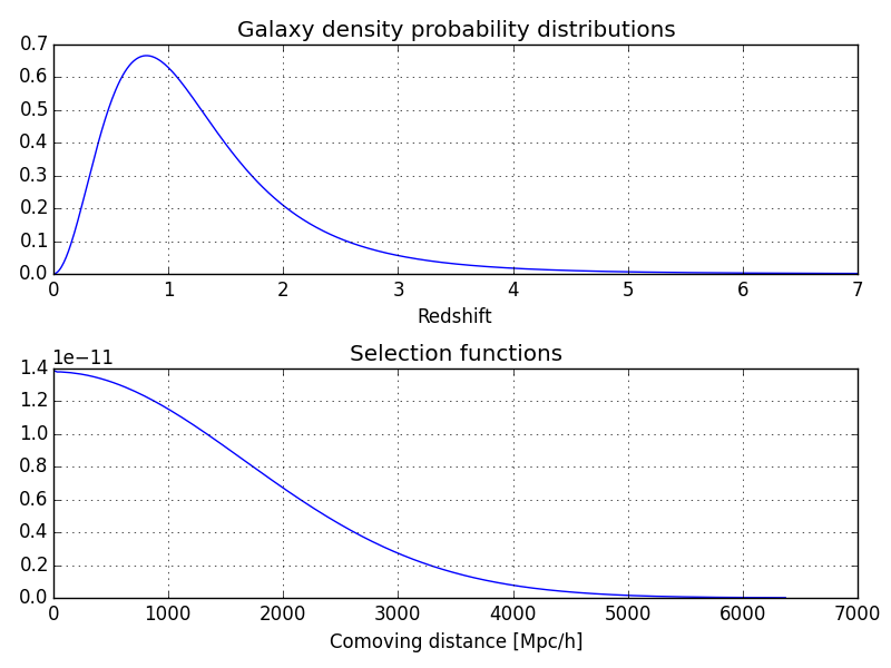
Below, we plot the selection function along with the normalized galaxy density distribution:

In [10]: z = arange(0.001,7.0,0.01)

In [11]: pz = surv.nz(z)

In [12]: r = cosmo.a2chi(z2a(z))     # Convert redshift array into comoving distance

In [13]: phi = surv.phi(cosmo,r)     # Compute selection function for both survey

In [14]: figure(); subplot(211);

In [15]: xlabel('Redshift'); grid(); title('Galaxy density probability distributions');

In [16]: plot(z,pz);

In [17]: subplot(212);

In [18]: xlabel('Comoving distance [Mpc/h]'); grid();  title(r'Selection functions');

In [19]: plot(r,phi);

Computing 3D power spectra¶

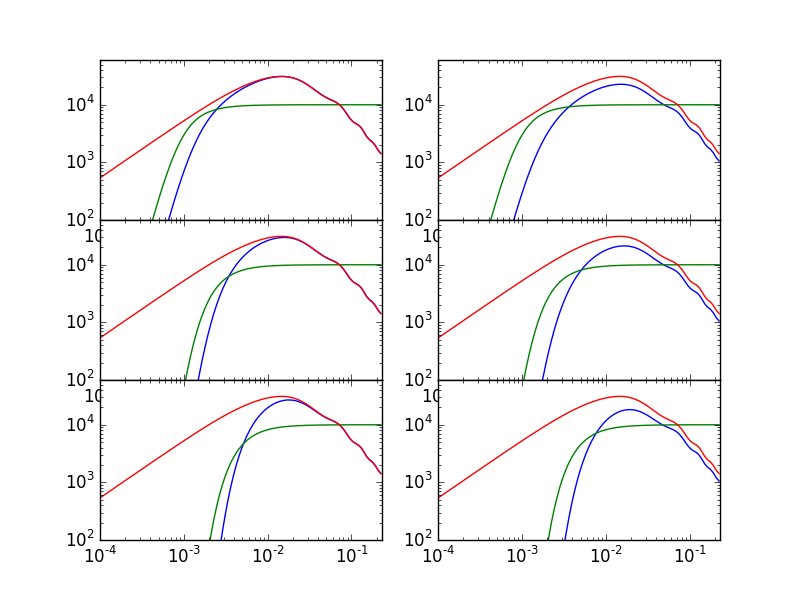
In [20]: sp = spectra(cosmo,surv)

In [21]: l = [2, 5, 10]             # Array of angular multipoles

In [22]: k = logspace(-4,-0.65,100) # Array of wavenumbers

In [23]: cl = sp.cl_sfb(l,k,shotNoise=False,evol=False)*(survey_volume**2)/r0*(2*sqrt(2*pi))

In [24]: cl_evol = sp.cl_sfb(l,k,shotNoise=False,evol=True)*(survey_volume**2)/r0*(2*sqrt(2*pi))

In [25]: cln = sp.cl_sfb(l,k,onlyNoise=True)*(survey_volume**2)/r0*(2*sqrt(2*pi))

In [26]: figure(); subplot(321);

In [27]: loglog(k,cl[0,:]); loglog(k,cln[0,:]); loglog(k,cosmo.pk_lin(k));

In [28]: ylim(1e2,6e4); xlim(0.0001,0.23);

In [29]: subplot(323);

In [30]: loglog(k,cl[1,:]);  loglog(k,cln[1,:]); loglog(k,cosmo.pk_lin(k));

In [31]: ylim(1e2,6e4); xlim(0.0001,0.23);

In [32]: subplot(325);

In [33]: loglog(k,cl[2,:]); loglog(k,cln[2,:]); loglog(k,cosmo.pk_lin(k));

In [34]: ylim(1e2,6e4); xlim(0.0001,0.23);

In [35]: subplot(322);

In [36]: loglog(k,cl_evol[0,:]); loglog(k,cln[0,:]); loglog(k,cosmo.pk_lin(k));

In [37]: ylim(1e2,6e4); xlim(0.0001,0.23);

In [38]: subplot(324);

In [39]: loglog(k,cl_evol[1,:]); loglog(k,cln[1,:]); loglog(k,cosmo.pk_lin(k));

In [40]: ylim(1e2,6e4); xlim(0.0001,0.23);

In [41]: subplot(326);

In [42]: loglog(k,cl_evol[2,:]); loglog(k,cln[2,:]); loglog(k,cosmo.pk_lin(k));

In [43]: ylim(1e2,6e4); xlim(0.0001,0.23);

In [44]: subplots_adjust(hspace=0);

References¶

[YooDesjacques13]

J. Yoo and V. Desjacques. All-sky analysis of the general relativistic galaxy power spectrum. PhysRevD, 88(2):023502, July 2013. arXiv:1301.4501, doi:10.1103/PhysRevD.88.023502.